- Telecommunications
- Systems & infrastructure
- Development & tooling
Monitoring a satellite’s emissions with Grafana
A dashboard that shows when a satellite channel transmits, rebuilds its spectrum in one click and calculates its emission rate over any period
Summary
My department at Airbus Defence and Space monitors the radio emissions of a satellite’s communication channels. Its monitoring application receives the measurements in real time, but it lacks three features the team needs: displaying the spectrum of a chosen moment, setting an emission threshold, and calculating an emission rate. I designed and built a Grafana dashboard that adds them. It reads the measurements from the InfluxDB database, plots the carrier power over a chosen period, rebuilds the frequency spectrum of any moment in one click, and calculates the emission rate against a threshold that follows the channel: its average power outside transmissions, plus a margin chosen from a drop-down menu. It stays responsive over long periods, and it comes with technical documentation and a user guide for the teams.
Written as a technical report, with the structure taught in ENSEEIHT’s written-communication course: a summary, an introduction, four numbered parts, a conclusion and the sources.
Confidential project: the equipment, the software and the frequencies are not named, and every value, screen and example on this page is fictitious.
1. Introduction
My department at Airbus Defence and Space works on a satellite communications project. The satellite carries several communication channels, and the team needs to know, for each one, when it transmits and what its signal looks like.
The measurements of every channel arrive in real time in a monitoring application, which stores them in an InfluxDB database [2]. This application is very complete, but it lacks some features the team needs for its analyses. My manager asked me to add them with a Grafana dashboard [1].
The question
How can the team see, for any channel and any period, when it transmits, what its spectrum looks like at a given moment, and what share of the time it transmits?
Objectives
- Plot the carrier power of a channel over a period the user chooses.
- Rebuild the frequency spectrum of the moment the user clicks on.
- Set the threshold above which the channel counts as transmitting: its average power outside transmissions, plus a margin the user chooses.
- Calculate the emission rate automatically over the chosen period.
Part 2 describes what the monitoring application lacks. Part 3 explains the method and the technical choices, panel by panel. Part 4 presents the results, and part 5 analyses them and proposes next steps.
2. What the monitoring application lacks
The monitoring application receives every measurement and stores it in InfluxDB. It shows the state of each channel, but three features are missing for the team’s analyses:
-
A spectrum on demand
Selecting a moment on a graph of the carrier power does not display the spectrum of that moment.
-
An adjustable threshold
Nothing lets the team decide from which power level a channel counts as transmitting.
-
An emission rate
Nothing calculates the share of time a channel spends transmitting over a period.
The dashboard reads the database that the application already fills. The acquisition chain stays untouched: the dashboard writes nothing.
3. Four values, three panels: method and choices
The work follows the path of the data: from the acquisition chain to the database, then from the database to each panel.
3.1 Where the data comes from
The signal received from the satellite reaches a digitiser, which converts it from analogue to digital. The monitoring application collects the measurements of each channel and writes them to InfluxDB 1.8, with the Flux language enabled (Figure 1).
The dashboard reaches this database through two data sources: the InfluxDB source, queried in Flux, and the Infinity source [3], which sends HTTP requests and processes their JSON answers.
3.2 The values used
Each measurement holds many fields. The dashboard needs only four:
| Value | What it is | Used for |
|---|---|---|
cp | Carrier power, in dBm | Power over time, emission rate |
powerdBm | The power values across the channel, in dBm, stored as one list | Spectrum |
startFreqHz | The frequency of the first value of that list, in Hz | Spectrum |
deltaFreqHz | The frequency step between two values of the list, in Hz | Spectrum |
The queries read only these values: the other fields never leave the database.
3.3 Panel by panel
Carrier power over time
- Need
- See when a channel transmits.
- How
-
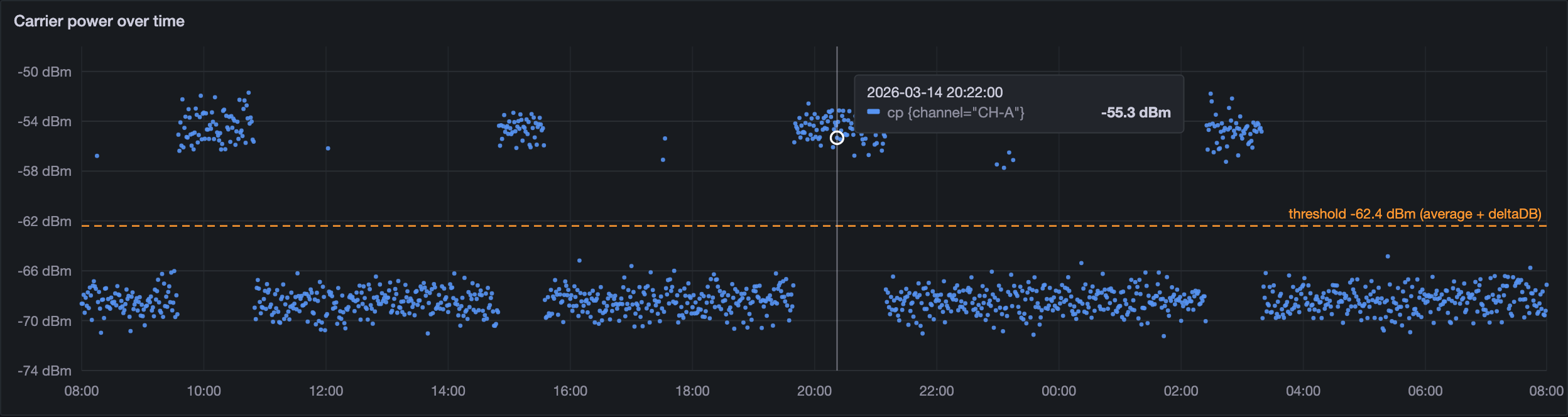
A Flux query reads the cp values of the selected channel over the chosen period. When the period is long, specific conditions in the query reduce the calculation load before the points reach Grafana. Their details stay confidential.
- Result
- Transmissions stand out above the noise, and the user can zoom on any part of the period (Figure 2).
The spectrum of a chosen moment
- Need
- Check what the signal looks like when a point stands out.
- How
-
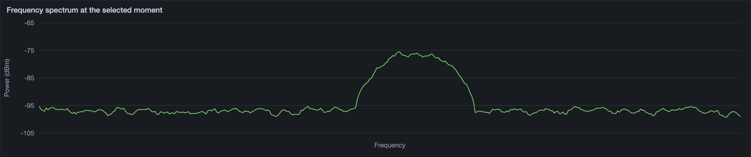
A click on a point of the time graph stores its timestamp in a dashboard variable, clicked_ts. The Infinity source then sends an InfluxQL query over HTTP: it fetches the last measurement of the channel at or before that moment (Listing 1). The answer is a JSON array. A UQL script [4] splits the list of powers into numbers and gives each value its frequency with equation (1), where i is the position of the value in the list.
SELECT powerdBm, startFreqHz, deltaFreqHz
FROM channel_measurements
WHERE carrier = '${channel}'
  AND time <= ${clicked_ts}ms
ORDER BY time DESC
LIMIT 1
Listing 1 – The spectrum query, in InfluxQL (names made generic) frequency(i) = startFreqHz + i × deltaFreqHz (1)
Example with fictitious values: with startFreqHz = 5,000 Hz and deltaFreqHz = 50 Hz, the first three powers sit at 5,000, 5,050 and 5,100 Hz.
- Result
- Each power value is paired with its frequency, and the spectrum appears under the time graph (Figure 3).
The emission rate
- Need
- Know what share of the time a channel transmits.
- How
-
The threshold follows the channel. The dashboard calculates the average carrier power outside transmissions over the period: the noise level of the channel. The user adds a margin in dB, chosen from a drop-down menu at the top of the dashboard (the deltaDB variable). Equation (2) gives the threshold. A Flux query then compares every cp value of the period with this threshold and counts the points above it: the points “in emission”. Equation (3) gives the rate.
threshold (dBm) = average power outside transmissions (dBm) + deltaDB (dB) (2)
emission rate (%) = (points in emission ÷ all points) × 100 (3)
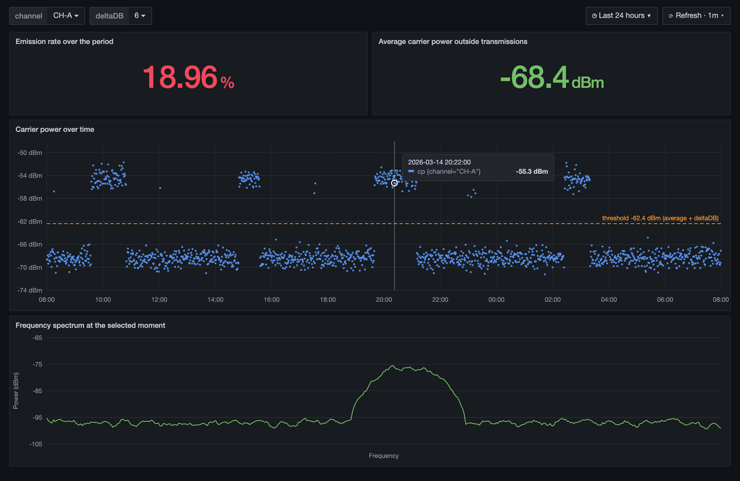
Example with the fictitious values of Figure 4: with an average of −68.4 dBm and deltaDB = 6 dB, every point above −62.4 dBm counts as in emission.
- Result
- The threshold and the rate update as soon as the period, the channel or the margin changes.
3.4 Choices and reasons
| Choice | Reason |
|---|---|
| Build on the existing database | The dashboard only reads: the acquisition chain and the application stay untouched. |
| Flux for the time graph and the rate | The comparison and the count run in the database: only the result travels to Grafana. |
| Lighter queries on long periods | The calculation load stays reasonable, and the dashboard stays usable over days of data. |
| Infinity and UQL for the spectrum | The powers are stored as one list. UQL turns a simple InfluxQL query into a full spectrum, inside Grafana, with no extra service. |
| A threshold tied to the noise level | Each channel gets a threshold that matches its own noise level; the deltaDB margin only sets how strict it is, in one click. |
4. Results: the three missing features are delivered
Figure 4 shows the finished dashboard. At the very top, the channel and the deltaDB margin, chosen from drop-down menus. Below them, the emission rate and the average carrier power outside transmissions, on which the threshold is based. In the middle, the carrier power over the chosen period. At the bottom, the spectrum of the selected moment.
-
3 of 3
missing features delivered
A spectrum on demand, an adjustable threshold, an automatic emission rate.
-
1 click
from a point in time to its spectrum
The timestamp of the point drives the query.
-
4
values read from each measurement
Out of the many fields each measurement holds.
-
2
documents for the teams
Technical documentation and a step-by-step user guide.
Delivered
- The dashboard, with two drop-down variables: the channel and the deltaDB margin
- Technical documentation that explains every query and every calculation
- A procedure that guides the teams, step by step, through using the dashboard
5. Analysis and next steps
What works well
- It meets the need without changing anything in the acquisition chain: it only reads the database.
- The spectrum is rebuilt from the measurement itself, so it matches the selected moment exactly.
- The threshold follows the noise level of each channel, so the same dashboard serves every channel; the user only chooses the margin.
Limits, and what I would do next
-
The margin is chosen by hand
Too small, it counts noise peaks as emissions; too large, it misses the weakest ones.
Next step: Suggest the margin from the spread of the noise, for example a multiple of its standard deviation, or learn it from emissions already confirmed.
-
One moment at a time
The spectrum shows a single moment: comparing two moments means switching between them.
Next step: Show two spectra side by side, or a waterfall: the spectrum over time, as a colour map.
-
Someone has to look
The dashboard shows the emissions, but it warns no one.
Next step: Grafana alerts when a channel transmits outside its expected windows; later, a model trained to spot unusual emissions, where AI helps to watch over a system.
Conclusion
The dashboard answers the question set at the start. For any channel and any period, the team sees when the channel transmits, displays its spectrum at any moment in one click, and reads its emission rate against a threshold that follows the channel’s noise level. It does so without changing the monitoring application, by reading the database the application already fills.
I carried the project from the need to the documentation: the queries in Flux and InfluxQL, the processing in UQL, the dashboard itself, and the documents that let the teams use and maintain it. The next steps would be a margin suggested automatically and alerts on unusual emissions.
The project lasted several months and put many of my skills to the test: organising my work, developing, testing, improving. It taught me to start from what users lack, to justify each technical choice, and to write documentation that others can rely on.
Sources
- [1] Grafana Labs, “Grafana documentation”, grafana.com/docs/grafana/latest/ (opens in a new tab)
- [2] InfluxData, “InfluxDB 1.8 documentation”, docs.influxdata.com/influxdb/v1/ (opens in a new tab)
- [3] Grafana Labs, “Infinity data source plugin”, grafana.com/docs/plugins/yesoreyeram-infinity-datasource/latest/ (opens in a new tab)
- [4] Grafana Labs, “UQL”, in the Infinity data source documentation, grafana.com/docs/plugins/yesoreyeram-infinity-datasource/latest/query/uql/ (opens in a new tab)
Terms
- dBm
- A power in decibels relative to one milliwatt. −60 dBm is a million times weaker than 0 dBm. A difference between two powers in dBm is in dB: the unit of deltaDB.
- Carrier power
- The power of the signal that carries a channel. It rises clearly above the noise when the channel transmits.
- Frequency spectrum
- The power of a signal frequency by frequency, at a given moment.
- Flux and InfluxQL
- Two query languages for InfluxDB: Flux can filter, calculate and aggregate in the database; InfluxQL is close to SQL.
- UQL
- The query language of Grafana’s Infinity data source, used to reshape a JSON answer before it is displayed.
Skills demonstrated
Each skill links to the skills map on the Projects tab.